
Deep Learning with WASI Simulation Data for Estimating Chlorophyll a Concentration of Inland Water Bodies


Institute of Photogrammetry and Remote Sensing, Karlsruhe Institute of Technology, 76131 Karlsruhe, Germany
*
Author to whom correspondence should be addressed.
†
These authors contributed equally to this work.
Remote Sens. 2021, 13(4), 718; https://doi.org/10.3390/rs13040718
Submission received: 30 December 2020
/
Revised: 8 February 2021
/
Accepted: 9 February 2021
/
Published: 16 February 2021
(This article belongs to the Special Issue Remote Sensing of Water Resources Monitoring, Parametrization and Modeling)
Abstract
:Information about the chlorophyll a concentration of inland water bodies is essential for water monitoring. This study focuses on estimating chlorophyll a with remote sensing data, and machine learning (ML) approaches on the real-world SpecWa dataset. We adapt and apply a one-dimensional convolutional neural network (1D CNN) as a deep learning architecture for the first time to address this estimation. Since such a DL approach requires a large amount of data for its training, we rely on simulation data generated by the Water Color Simulator (WASI). This simulation is prepared accordingly and includes a knowledge-based water composition with two origins of the chlorophyll a concentration. Therefore, the training data is independent of the real-world SpecWa dataset, which is challenging for any ML approach. We define two spectral downsampling approaches as a pre-processing step, representing the hyperspectral EnMAP satellite mission (SR-EnMAP) and the multispectral Sentinel-2 mission (SR-Sentinel). Subsequently, we train a Random Forest, an artificial neural network, a band-ratio approach, and the 1D CNN on the WASI-generated simulation training dataset. Finally, all ML models are evaluated on the real SpecWa dataset. For both downsampled data, the 1D CNN outperforms the other ML models. On the finer resolved SR-EnMAP data it achieves an , μg L−1, and μg L−1. Besides, the 1D CNN’s performance decreases on the SR-Sentinel data to . When focusing on the individual water bodies of the SpecWa dataset, the most significant differences exist between natural and artificial water bodies. We discover that the applied models estimate the chlorophyll a concentration of most natural water bodies satisfyingly. In sum, the newly DL approach can estimate the chlorophyll a values of unknown inland water bodies successfully, although it is trained on an entire simulation dataset.
1. Introduction
1.1. Focus of This Study and Background
Remote sensing (RS) techniques have vast potential for monitoring the water quality of inland water bodies (see, for example, [1,2]). These techniques provide three main advantages over point-based in-situ water quality measurements due to the applicability of satellite data [1,2,3]. First, RS satellite data are recorded automatically, regularly, and frequently. Second, because of these frequent recordings, they are cost-efficient in the long-term. Third, satellite data cover a large spatial area with a single image, allowing exhaustive monitoring of inland water bodies. However, spectral RS techniques cannot measure water quality directly. The information in the spectra has to be extracted and transformed into water parameter values. These corresponding transfer approaches rely on statistical or data-driven models or physical models.
In the last decades, many studies have analyzed RS applicability with a particular focus on inland waters. Parameters retrieved from spectral RS data are chlorophyll a [4,5,6,7,8], colored dissolved organic matter (CDOM) [9], turbidity [10,11], total suspended solids [12,13], Secchi depth [14], and a distinction between different algae species, primarily cyanobacteria [15,16]. Regular recording of these parameters with low effort would benefit the work of the authorities in environmental concerns. In this context, satellite systems such as the Sentinel-2 and Sentinel-3 mission, launched in 2015 and 2016, provide data for a more frequent monitoring solution. Among the mentioned water parameters, chlorophyll a belongs to the most prominent ones [17]. Several studies focus on chlorophyll a retrieval based on the mentioned satellite data (see, for example, [18,19,20,21]). Chlorophyll a originates from phytoplankton and is a measure for the primary production and the biomass of a water ecosystem. Based on the chlorophyll a concentration, information about algae abundance, water quality, or nutrition supply of a water body can be concluded [22,23]. For example, this information is crucial for understanding and evaluating changes in ecosystems [24].
When estimating chlorophyll a values with RS data, approaches have to bridge the gaps between the spectral signature of chlorophyll a and the actual value of its concentration in inland waters. In general, two distinct approaches exist to retrieve water parameter values from the spectral RS data: analytical and empirical approaches [1]. As a kind of physical modeling approach, the former relates RS data with the underwater light field and the water quality properties. Analytical approaches are based on the inherent optical properties (IOPs) of the water constituents [25]. For a particular wavelength, the IOPs describe the underwater light field. Absorption coefficients, combined with scattering and backscattering coefficients of the water constituents, reveal the IOPs of a water column. The IOPs are physically related to the subsurface irradiance reflectance, the sun, as well as atmospheric conditions, which are linked to RS data via radiative transfer models [12,26,27,28]. Hence, the IOPs are quasi-independent of changing illumination conditions [29]. For example, the Water Color Simulator (WASI) [30] is a freely available tool providing and combining several analytical models to simulate different RS measurement quantities such as radiance reflectance. After selecting several models and parameter values, WASI provides a spectrum for the selected configuration.
Empirical approaches link the spectral RS data and the water parameters statistically. These approaches comprise feature engineering approaches (see, for example, [5,6,7,8,31]) such as band ratios (BR) and solely data-driven machine learning (ML) approaches. BR approaches commonly include a selection of spectral bands that are physically related to the target parameter, combined with linear regression to estimate water parameters. They achieve robust estimation results and are often applied but are limited, for example, concerning the generalization from one known water body to another unknown water body. Neil et al. [32] propose different BR approaches to overcome the generalization limitations of commonly applied BR approaches. They adapt and apply selected BR approaches on the 13 optical water types according to Spyrakos et al. [33], which perform better in estimating the chlorophyll a concentrations compared to approaches with the original parametrization.
ML approaches can learn the linkage between spectral input data and desired chlorophyll a values during a training process in existing datasets [34]. Learning this linkage is challenging since the water body’s spectral signature is defined by overlapping information of distinct water compositions. The applied data-driven approaches include shallow learners such as tree-based models, artificial neural networks (ANN) [35,36,37,38,39] and, recently, deep learning (DL) approaches. Convolutional neural networks (CNNs) are one type of DL models. For example, they have been applied by Syariz et al. [40], Pu et al. [41] to either estimate chlorophyll a concentrations based on RS satellite data or to predict the water quality of different discrete classes. However, current studies only focus on the estimation and classification task for one single water body. Therefore, these studies do not cover temporal changes over a season of the water composition and the chlorophyll a concentration and the variation of this concentration between individual inland water bodies.
To provide a first step towards more generalized ML approaches, Maier and Keller [42] rely on measured data of several water bodies instead of one water body’s data. During the training phase, the ML models learn on a data subset containing a selected subset of spectral data and chlorophyll a values of the underlying water bodies. Pahlevan et al. [21] also focus on in-situ spectrometer data of several lakes. They propose and implement a mixture density network, as a kind of shallow ANN, which is scaled to the respective satellite mission’s spectral resolution. This approach can estimate water parameters with real RS satellite data.
No DL approach to estimate chlorophyll a, which is trained on a data selection of inland waters and evaluated on a distinct, real-world dataset of entirely different water bodies, has been conducted to the best of our knowledge.
1.2. Motivation, Objectives, and Contributions
Our study is motivated by this generalization challenge concerning the chlorophyll a estimation. Therefore, we aim at estimating chlorophyll a values of several inland water bodies by applying purely data-driven ML approaches on RS data. In this context, we further investigate the potential of deep learning approaches, which have not yet been applied to estimate the chlorophyll a values. This intention naturally leads to the following but intriguing questions: Can ML approaches be trained on a simulated dataset to estimate the chlorophyll a concentration of water bodies not included in the training process? To address this overall question, we rely on the freely available SpecWa dataset [43]. It contains remotely recorded spectrometer data and point-based measured chlorophyll a values of eleven different inland water bodies in Germany covering small areas. We downsample the spectrometer data to hyperspectral and multispectral satellite resolution to evaluate the study’s contribution concerning inland water monitoring.
The simulated dataset is generated by applying the analytical WASI tool [29] with varying water parameters to map different water bodies and configurations. Note that we rely on the freely available WASI as an alternative to the commercial HydroLight [44]. As a result, we gain a large simulated dataset that we use to train different ML models. After the training process, these ML models are applied to the SpecWa dataset. The SpecWa dataset is so far unknown to the ML models. Using these two different datasets for training and test, the development of ML models handling the underlying estimation tasks is challenging. However, it ensures the procedure necessary for the generalization abilities of the ML models.
To solve this advanced estimation task, we rely on a one-dimensional convolutional neural network (1D CNN) as a new DL approach in this field of application. Such a 1D CNN has shown promising results in analyzing spectral data in the environmental classification task [45], which is one reason to rely on it in our estimation task. A random forest (RF) model [46] provides the baseline since it has already achieved good performance in estimating chlorophyll a concentrations of inland waters [47]. Besides, we also apply a common BR approach combined with linear regression.
Concerning the mentioned aspects and challenges, our main contributions linked to the study’s objective are:
- the development of a DL approach for estimating chlorophyll a concentrations of different inland water bodies inspired by a 1D CNN architecture;
- a detailed investigation and evaluation of the potential of this approach concerning the generalization aspects on unknown datasets;
- the comparison of the estimation performance of 1D CNN with a commonly applied ANN, RF and BR approach.
In Section 2, we briefly describe the SpecWa dataset and the simulated dataset based on the WASI tool. The preprocessing and splitting of the datasets is summarized in Section 2.4. We describe the applied ML approaches and the architecture of the 1D CNN in Section 2.5. The estimation results are presented in Section 3. Subsequently, we assess and evaluate the performance of applied ML models concerning the distinct spectral resolutions and the approaches’ generalization abilities (Section 4). In Section 5, the presented study is concluded, combined with an outlook of future studies.
2. Data and Methods
Before developing the methodology, it is essential to outline the prerequisites (see Section 2.1) relevant to the approach. It will then become apparent why we design the databases and the methodology, as presented in Section 2.2, Section 2.3, Section 2.4 and Section 2.5.
2.1. Requirements for DL Approaches
Since chlorophyll a is a continuous parameter, the task is to estimate its concentration. To solve this task, we have applied different ML approaches in recent studies (see, for example, [47,50,51]). In general, the selected approaches are defined by the available reference data, their quality, and the amount of available data. Concerning the estimation task, we rely on the SpecWa dataset as a real-world dataset. In contrast to Maier and Keller [37,42], we aim to estimate the chlorophyll a values of the SpecWa dataset without using these real-world data for the training process of the selected ML approaches. Therefore, further data are needed for the training, which we simulate with the WASI tool. This simulation offers the opportunity to generate a large dataset that enables us to apply a DL approach. Such an approach has not yet been used in the context of inland water monitoring with spectral data.
The DL approach is supposed to be applied to (a) a wide variety of inland water bodies resulting in heterogeneous input and reference data, (b) different spectral resolutions, and (c) for monitoring purposes of distinct inland water bodies. Since we aim at fulfilling these prerequisites, the data and their preparation need to meet the following four conditions:
- Number of datapoints: Many datapoints are needed to apply and train the DL models.
- Variety of water parameters: a combination of different water parameters is necessary since the ML models need to link different spectra (spectral input data) with different chlorophyll a values while these spectra are also characterized by signatures of other water parameters (“unmixing”). These occurring water parameters are, for example, CDOM, suspended materials, the consistency of the water bodies’ benthic substrate, and different algae species with different pigments. Besides, atmospherical effects and different radiation conditions during a day or a year are also considered.
- Value range of the target variable: To avoid dataset shift, the value range of the chlorophyll a values as desired target variable should be similar to the value ranges of many inland water bodies, and especially of the SpecWa dataset’s chlorophyll a values.
- Spectral distribution of the input data: The WASI-simulated spectral input data need to be in a similar distribution as the spectral data of the SpecWa dataset. Besides, as a pre-processing step, the WASI-simulated spectral data have to be scaled to the same spectral resolution as the SpecWa dataset to ensure compatibility.
2.2. Data Characteristics of the SpecWa Dataset
The SpecWa dataset consists of spectrometer measurements and in-situ water quality measurements on eleven different small-scale inland water bodies in the region around Karlsruhe, Germany, during the years 2018 and 2019. The spectral data have been measured with the RoX spectrometer (JB Hyperspectral). This sensor records the upwelling radiance from the water body and the downwelling irradiance of the atmosphere simultaneously. Its integration time is regulated by the upwards looking end with a cosine receptor at its top, leading to relatively stable measurements. Details of the measurement setup, such as the geographic position of the selected water bodies, are given in [43]. Eventually, the measured spectral data contain radiance reflectance values as a sum of water-leaving radiance and the surface reflectance. The chlorophyll a concentrations and the values of the other water parameters have been recorded in-situ by either the Algae Torch or the Algae Lab Analyzer (both manufactured by bbe moldaenke) in a depth of 20 cm below the water surface. The SpecWa dataset consists of 3685 datapoints with the spectral data in the range of 389 nm to 910 nm and the respective chlorophyll a value as a reference.
Table 1 shows the essential information of the SpecWa dataset, including the ID designation of the water bodies. For this study, we rely on datapoints with the following two characteristics concerning specific water parameters:
- datapoints with a chlorophyll a concentration lower than 100 μg L−1 are included;
- datapoints with a cyanobacteria concentration lower than 5 μg L−1 are included.
We must constrain the dataset to ensure the compatibility of the WASI-generated simulation data and avoid possible dataset shifts and resulting suffering of the estimation performance [52,53]. Note that the WASI tool can only generate reliable data for the mentioned chlorophyll a concentrations, whereas cyanobacteria are not implemented. In sum, we receive a reduced SpecWa dataset with 2617 datapoints and 801 spectral bands (spectral features). We use this dataset later as the eventual test dataset for the ML approaches. Figure 1 and Table 1 provide an overview of the chlorophyll a distribution in the final SpecWa dataset. Besides, Figure 2 shows the spectral data of two selected water bodies concerning the means and the standard deviations.
2.3. Fundamentals of the WASI Tool and Simulation of the WASI Data
The WASI tool is a sensor independent water spectra generator and analyzer. We can use WASI to calculate radiance reflectance or other spectral data based on a number and combination of possible input parameters as modifiable variables [29]. We can either calculate a spectrum for the given input parameters or use WASI to estimate water parameters based on, for example, a least-square fit with multiple iterations and parameters [54]. We can also select different physical or analytical models to simulate the optical path from the sun through the water to the sensor. The spectral signatures can be read in from files for different parameters such as algae species, or bottom reflectance spectra with different constituents. In this study, we apply the WASI tool to generate simulated spectra with a specific combination of variables and chlorophyll a values.
Therefore, the input data structure of the WASI-generated simulation data needs to be similar to the SpecWa data structure. In our case, the spectral data of the SpecWa dataset is given in radiance reflectance (see [43]). The radiance reflectance is the sum of the water leaving radiance and the reflectance on the water surface on a radiance sensor in proportion to the incoming irradiance [55,56]. Consequently, we simulate data with the WASI tool as radiance reflectance data by varying the input parameters. For our setup, the WASI tool provides 33 parameters that can be adapted for radiance reflectance, but only three parameters can be varied simultaneously. Besides, we select 12 out of the possible 33 WASI parameters which affect the water-leaving radiance and the surface reflectance. The remaining WASI parameters are set to default. Table 2 summarizes the 12 selected WASI parameters.
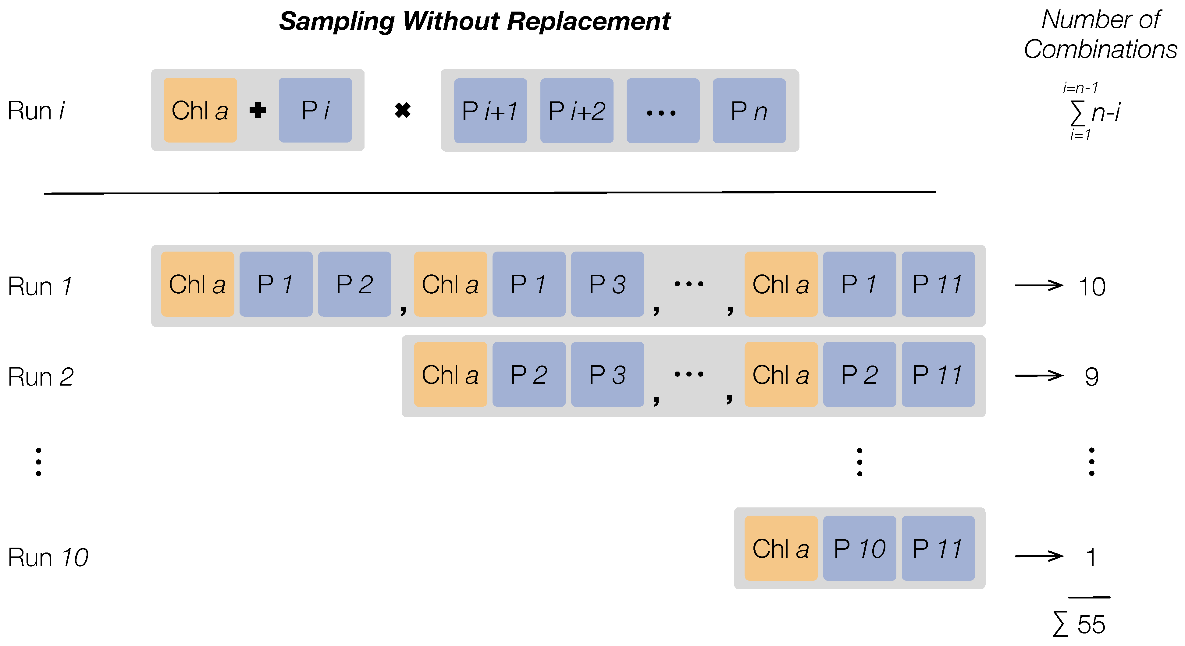
We define a sampling schema to handle the parameter combination, which is visualized in Figure 3. We include the chlorophyll a concentration as a parameter in every run and select two additional out of the remaining 11 parameters (see Table 2) in an iterative process as variable settings. Since we aim to cover every combination of the parameters and the chlorophyll a concentration, we receive 55 WASI-parameter combinations in 10 runs, as shown in Figure 3.
In each run, we consider the selected three parameters’ value range and their frequencies’ distribution (see Table 2, range and steps column). Both, the range and the frequency, are selected according to the following two criteria: (i) We use the range of the respective parameter so that a wide variety of possible inland water bodies is represented. (ii) In addition, we simulate the respective parameter value’s frequency so that it is nearly equally or logarithmically equally distributed. This distribution is crucial to ensure that the DL approaches are provided with the full range of the data and not only the majority.
The remaining WASI parameters, which are not among the selected three parameters, are set to a constant value according to Table A1 in Appendix A. These constant values are also given in Table 2 at column Standard. The WASI-generated chlorophyll a data covers the range from 0.1 μg L−1 to 100 μg L−1 in 30 steps with a logarithmic step width in each run.
Since the chlorophyll a concentration depends on the green algae species and the diatom species, we simulate the sampling schema twice. The first time, green algae represent the varying chlorophyll a concentration and the diatom concentration is excluded; while the second time, it is vice versa.
Finally, we receive a number of 528,000 WASI-generated datapoints containing the radiance reflectance values in the range of 400 nm to 900 nm with a spectral resolution of 1 nm and varying values of the selected 12 parameters. For the chlorophyll a estimation, we consider only the spectral input data with a number of 501 bands (features) and the respective values of the chlorophyll a concentration. Figure 4 shows one example of the WASI-generated spectral data.
2.4. Data Pre-Processing
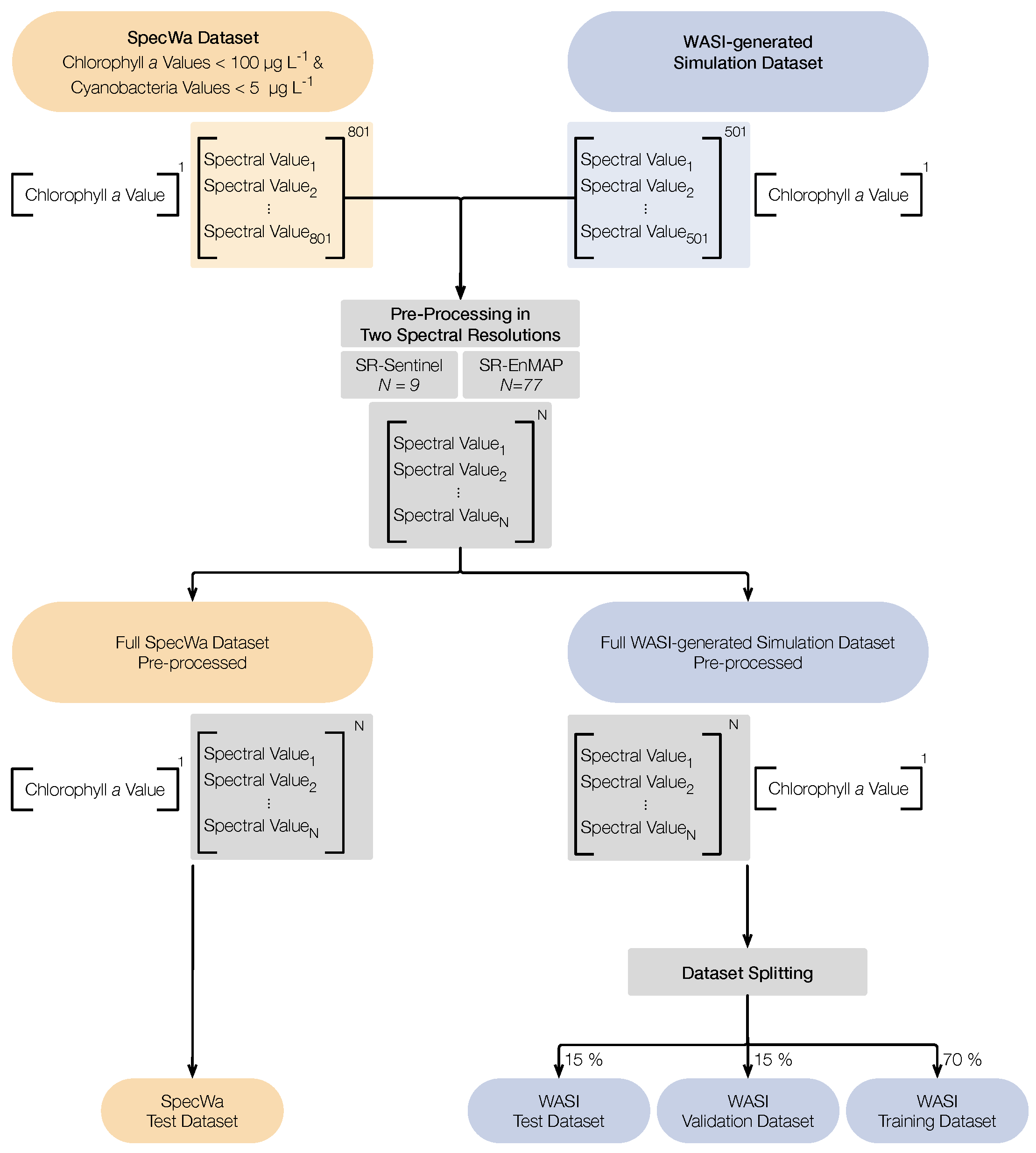
We apply two pre-processing steps. First, a standard spectral resolution of the SpecWa and the WASI-generated simulation data is needed (see Section 2.4.1). Second, the full WASI-generated simulation dataset needs to be split into smaller datasets to evaluate the applied ML models’ generalization abilities. This dataset splitting is described in Section 2.4.2, while the entire pre-processing workflow for all datasets is shown in Figure 5.
2.4.1. Downsampling
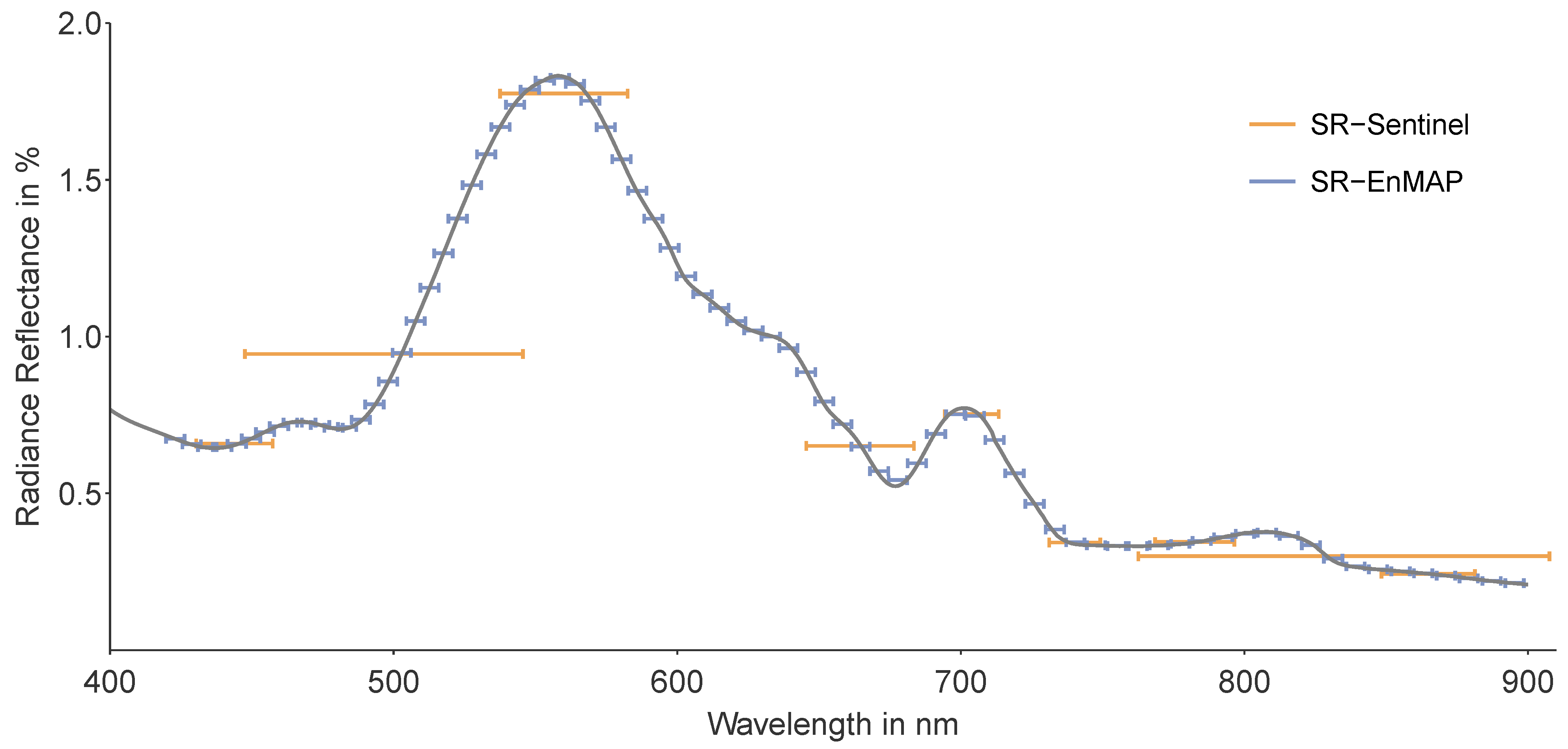
As demonstrated in Maier and Keller [42], the estimation performance of supervised ML models in terms of chlorophyll a is satisfying concerning different downsampled spectral resolutions (4 nm, 8 nm, 12 nm, 20 nm) of the input data. This study’s main finding is that finer resolved spectral features such as a 4 nm resolution do not improve the ML estimation performance since the spectral features are highly correlated. Additional downsampling is also conducted for the spectral resolution of satellite missions [57] in terms of BR-feature engineering approaches. Motivated by these studies and the goal to prepare an up-scaling approach on available spectral satellite data, we aggregate all spectral input features of the SpecWa dataset and the WASI-generated simulation dataset. This aggregation is conducted with the spectral resolution of the commonly applied multispectral Sentinel-2 mission (ESA) [49] and the upcoming hyperspectral EnMAP mission (DLR) [48]. The former results in 9 spectral features, while the latter generates 77 spectral features. Figure 4 visualizes the resulting spectral downsampling of the two applied resolutions. We refer to the spectral resolution of the Sentinel-2 mission as SR-Sentinel and of the EnMAP mission as SR-EnMAP. The spectral scaling is implemented in the R package hsdar provided by Lehnert et al. [58]. As for the simulated Sentinel-2 scaling, we apply the MSI instrument’s real spectral response function on Sentinel-2, while for the EnMAP downsampling, no spectral response function is available yet. Therefore, we use a Gaussian distribution around the central wavelength of each EnMAP-band as the weight for the input of the respective spectral channel, which is provided in the hsdar package. Note that the proposed downsampling data cannot be directly compared to atmospherically corrected multi- and hyperspectral data. The latter is characterized by additional noise due to atmospheric condition which is absent in the SpecWa data. Therefore, the ML approaches’ estimation performances on the downsampled, satellite-alike spectral features would certainly outperform an ML-based estimation based on satellite data concerning an area-wide upscaling monitoring approach.
2.4.2. Dataset Splitting in Subsets
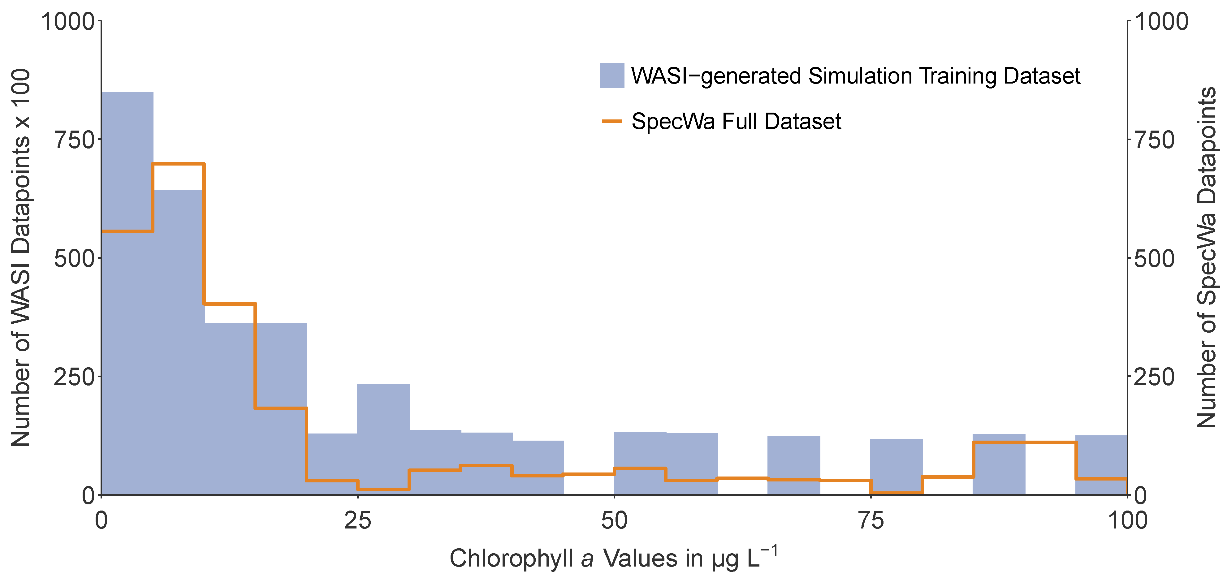
To evaluate the ML models’ performance, an independent splitting of the training dataset and test dataset is necessary. Therefore, we randomly split the WASI-generated simulation dataset into three sets (see Figure 5). The training dataset is used to train the ML model. The test dataset is solely used to evaluate the respective final ML model. Eventually, the validation dataset is used during the optimization process of the ML model to evaluate the generalization ability of the respective model. The ratio of the split into the three different datasets is presented in Table 3. We also consider the SpecWa dataset with a number of 2617 datapoints as a second test dataset since we aim to evaluate the estimation performance of the ML model on several unknown inland water bodies. Figure 6 shows the distribution of the chlorophyll a values between the WASI training subset and the SpecWa dataset as the final test dataset.
2.5. Machine Learning Models
Several supervised learning approaches exist using spectral input data to estimate environmental parameters, for example, chlorophyll a values. Among others, Keller et al. [47] rely on ten shallow learning techniques to estimate of distinct water parameters. Besides, Maier and Keller [37] investigate the effect of different spectral input data resolutions for the estimation task. Artificial neural networks are a powerful tool to predict variables with nonlinear relations (see, e.g., Hafeez et al. [39]). This finding is also met by Maier and Keller [37] on simulated Sentinel-2 resolution data. Other neural networks were applied by, e.g., Pahlevan et al. [21], González Vilas et al. [36], Chebud et al. [38], whereas Syariz et al. [40], Pu et al. [41] applied CNNs on Landsat 8 and Sentinel-3 images to classify or estimate water quality.
In this study, we evaluate several ML approaches for the challenging task of estimating chlorophyll a values based on two different spectral resolved input data and for water bodies excluded in the training process of the applied ML models. We select a Random Forest (RF) [37,39] as a shallow learning approach, an artificial neural network (ANN) [36,37,38,39], and an innovative one-dimensional convolutional neural network (1D CNN) [45,59] as a DL approach. Furthermore, we apply a feature-engineering approach combined with a linear regression called a band-ratio (BR) approach [31]. RF and the selected BR represent two commonly applied approaches when estimating the chlorophyll a concentration of inland water bodies. Thus, we compare the more sophisticated ANN and 1D CNN estimation performances against the results of the RF and the BR approach as baselines.
Since the RF has achieved sophisticated estimation performance in previous studies conducted on a subset of the SpecWa dataset (see [37,42]), we rely on it as a baseline. One particularity of the mentioned studies is that the RF shows better performance when it is applied on the first derivative of the spectral input data. Therefore, we also use the first derivative, calculated with the prospectr package in R [60], as input for the RF.
We rely on a feature engineering band-ratio (BR) approach in addition to the shallow RF model. This kind of approach is established in remote sensing applications for inland water bodies (see [31]). A three-band selection combined with a linear regression enables this BR approach to estimate the chlorophyll a concentration. The proposed bands, according to Moses et al. [31], are slightly adapted, since they are related to the MODIS and the MERIS sensor. In the case of the SR-EnMAP resolution, we select bands at 664.7 nm, 711.9 nm, and 755 nm, while in the case of SR-Sentinel resolution bands at 665 nm, 705 nm, and 740 nm are chosen. We parametrize the BR approach on the WASI-generated simulation training dataset with linear regression. Subsequently, we apply it to the WASI test dataset and the SpecWa test dataset, to ensure comparability.
Although CNNs are mainly popular in image understanding, they are recently used in remote sensing classification tasks based on spectral image data Liu et al. [59], Hu et al. [61], and spectral input data [45]. One strength of a 1D CNN architecture is that several features are generated from the spectral input data in the network’s deep layers. These features are kind of similar to the derivatives used as input for the RF. Besides, 1D CNN is more resistant to the noise of the input data. Noise can occur, for example, due to changing weather conditions during the measurements or variation in the calibration techniques. Figure 7 illustrates the 1D CNN architecture for the SR-EnMAP data. As for the smaller dimensioned SR-Sentinel input data, the 1D CNN architecture differs. The main differences between the 1D CNN hyperparameters of the two spectral simulated input data are given in Table A2. All hyperparameters are determined with an optimization process.
In the following, we describe the architecture of the 1D CNN for the SR-EnMAP simulated spectral data since this 1D CNN is more complicated than the 1D CNN for the SR-Sentinel simulated spectral data. This architecture is inspired by the LeNet5 network [62] and the LucasCNN [45] but is adapted to our specific estimation task, especially concerning the last layers. The final adaption is a result of the performance on the validation dataset. Our 1D CNN consists of four convolutional layers (CONV) with different filters and filter sizes (see Table A2). Each CONV layer is followed by a max-pooling layer (MaxPooling). After the final CONV layer, we place a flatten layer and a dropout layer (Dropout) with a dropout rate of 0.2 to counter overfitting. Before the end of the network, two fully-connected (FC) layers are implemented. We include a layer with Gaussian noise (Noise) to ensure a more stable DL model between these FC layers and again to avoid overfitting. The second and last FC layer is combined with a linear activation function to enable this 1D CNN to solve the underlying estimation task. Except for this last activation function, we rely on the commonly applied ReLU function [63]. The fitting of the network is conducted with the Adam optimizer [64]. Adam optimization is an extension of a stochastic gradient descent, which updates the CNN’s weights more efficiently by using momentum and adaptive learning rates to converge faster. We use the mean squared error as a loss function, a batch size of 256, and 100 epochs. Note that the dropout and noise layers exist only during the training of the 1D CNN.
In addition to the 1D CNN, we study a flatter ANN architecture (see Table A2). The ANN consists of an input layer, two hidden layers with 100 neurons each, and an output with one neuron. ReLu is used as an activation function in-between all these layers, except for the last single neuron. This neuron is activated with a linear function. Besides, we also apply a dropout layer and a noise layer similar to the 1D CNN.
All ML models are trained and evaluated ten times on different seeds to evaluate the stability of the models. The estimation performances of the different ML models are compared based on the coefficient of determination (), the mean absolute error (MAE), and the root mean square error (RMSE). As for the 1D CNN the best model of the training and validation process is selected to perform on the test and SpecWa test dataset.
3. Results
In the following, we present the chlorophyll a estimation results of the different ML approaches combined with the two downsampled resolutions, SR-EnMAP and SR-Sentinel. The 1D CNN, the ANN, and the RF performances on the WASI test dataset are greater than for the SR-EnMAP-data and for the SR-Sentinel-data, as expected since the WASI-generated simulation data is relatively homogeneous. Therefore, we focus on the estimation performance with the independent, real-world SpecWa dataset, representing the study’s primary objective. The results are structured in three parts: (1) We describe the applied models’ overall estimation results on the complete SpecWa dataset. (2) Subsequently, the best ML model is selected to investigate the estimation performance on the respective dataset in detail. (3) The specific estimations for the eleven water bodies of the SpecWa dataset are described.
Table 4 shows the overall estimation performance of the 1D CNN, the ANN, and the two baseline models, RF and BR, in terms of the three metrics , RMSE, and MAE, for the SpecWa (test) dataset. Concerning the two spectral resolutions, the 1D CNN and the ANN achieve better estimation results on the finely resolved SR-EnMAP data. At the same time, RF and BR perform better on the SR-Sentinel data for all performance metrics. Overall, the 1D CNN represents the best estimation model with , μg L−1, and μg L−1 on the SR-EnMAP data. The ANN performs as the second-best model on the SR-EnMAP data, but it is significantly worse than the 1D CNN. On the SR-Sentinel data, the 1D CNN is also the best model. However, in this case, the 1D CNN underperforms with an , μg L−1, and μg L−1 compared to its performance on the finely resolved SR-EnMAP data. Regarding the three estimation metrics and the SR-Sentinel, the 1D CNN’s performance is only better in the case of the -score compared to the RF. Otherwise, the range of the models’ performance metrics is smaller on the SR-Sentinel data. For example, the -score of all models ranges from 37.9% to 81.9% on the SR-EnMAP data, while -score varies from 51.5% to 62.4% on the SR-Sentinel. In order to compare the estimation results with the measured chlorophyll a values in the subsequent Section 4, we provide additional information about the SpecWa chlorophyll a values (see also Figure 1). The chlorophyll a ranges from 0 μg L−1 to 99.6 μg L−1 for all SpecWa inland water bodies with a mean value of 23.85 μg L−1 and a median value of 10.1 μg L−1. Based on this information, in sum, the results on the SR-Sentinel data remain unconvincing (see Table 4, right part) for all selected models.
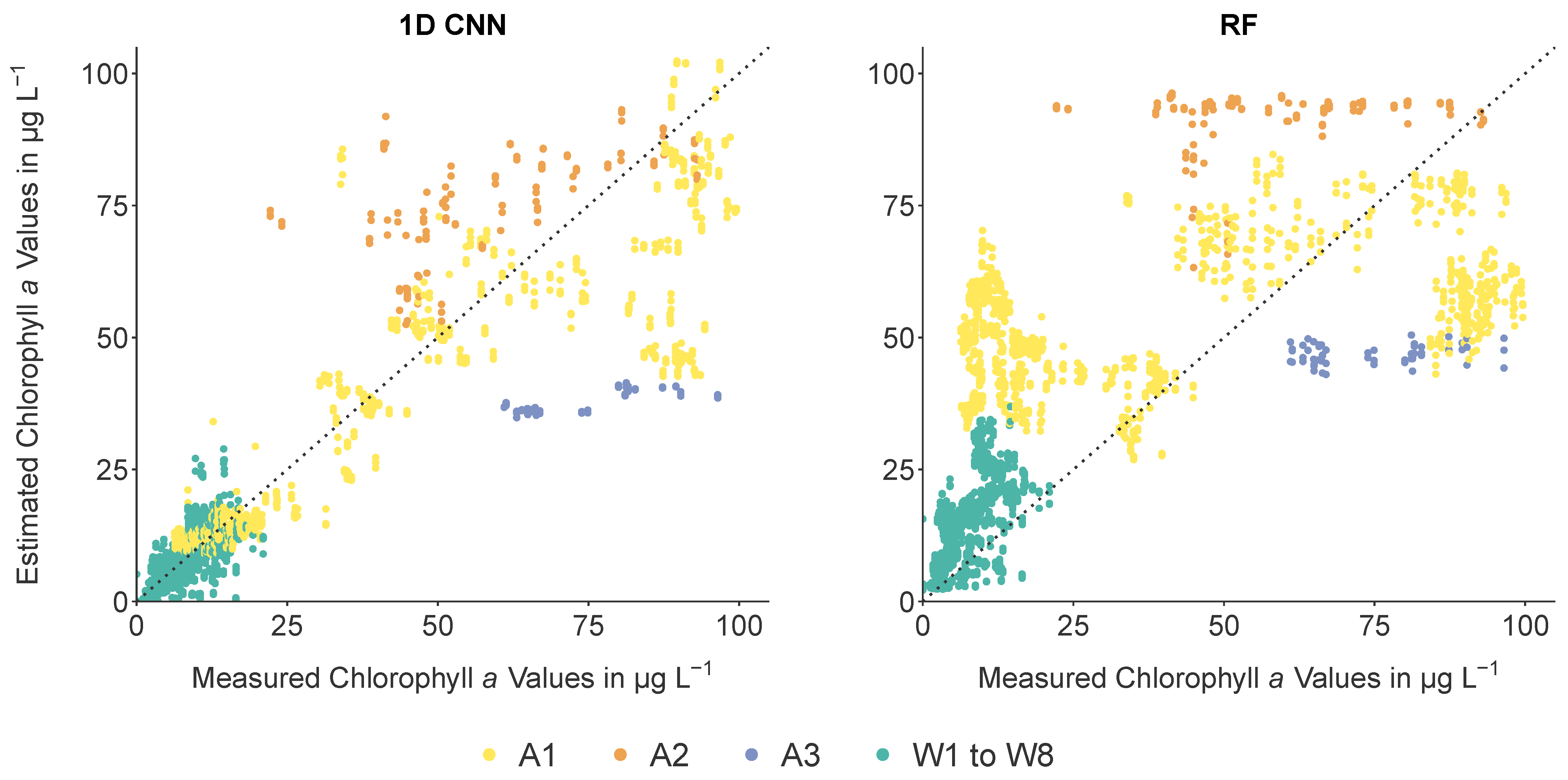
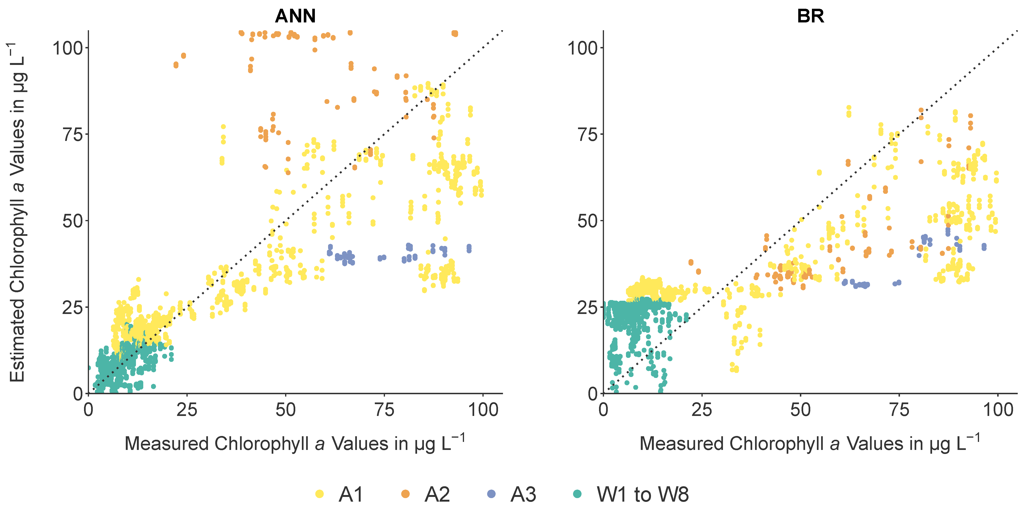
Since the 1D CNN represents the best model on the complete SpecWa dataset, especially for the SR-EnMAP data, we focus on its estimation performance in detail. Figure 8 (left) shows the results generated by the 1D CNN model compared to the measured chlorophyll a values on the SpecWa dataset. On the right of Figure 8, we provide the estimation results generated by the RF baseline compared to the measured chlorophyll a values on the SpecWa dataset. As for the visualized 1D CNN-generated distribution of the estimated and measured chlorophyll a values, we notice that most of the low values of the natural water bodies W1 to W8 are estimated correctly (low bias). The 1D CNN over- and underestimates a limited amount of datapoints. This finding is primarily related to higher chlorophyll a values. The chlorophyll a values of the water body A2 are consequently overestimated whereas the water body A3 values are underestimated. In contrast, the RF (Figure 8, right) shows a significantly worse distribution of the estimated and measured chlorophyll a values (high bias). The RF overestimates most of the SpecWa chlorophyll a values; solely the values of the water body A3 are underestimated. In addition, Figure A1 visualizes the estimation results generated by the ANN and the baseline BR.
With respect to a detailed analysis of the individual water bodies, we summarize the estimation performance of all selected ML models on each SpecWa water body in Figure 9 in terms of the RMSE, accompanied by the specific values for the MAE and RMSE in Table 5. Note that the -score is not provided. In the case of the individual inland water bodies, the number of datapoints is too low and the range of the chlorophyll a concentration is partly too small, resulting in inconclusive -values. The estimation results for the different water bodies can be sorted into three parts. The first part includes water bodies whose chlorophyll a values are generally well-estimated by several models independently of the two spectral resolutions. Secondly, water bodies exist whose chlorophyll a values are only well-estimated by a few models or only on one of the downsampled spectral resolutions. Furthermore, water bodies whose chlorophyll a values are generally hard to estimate by all ML models.
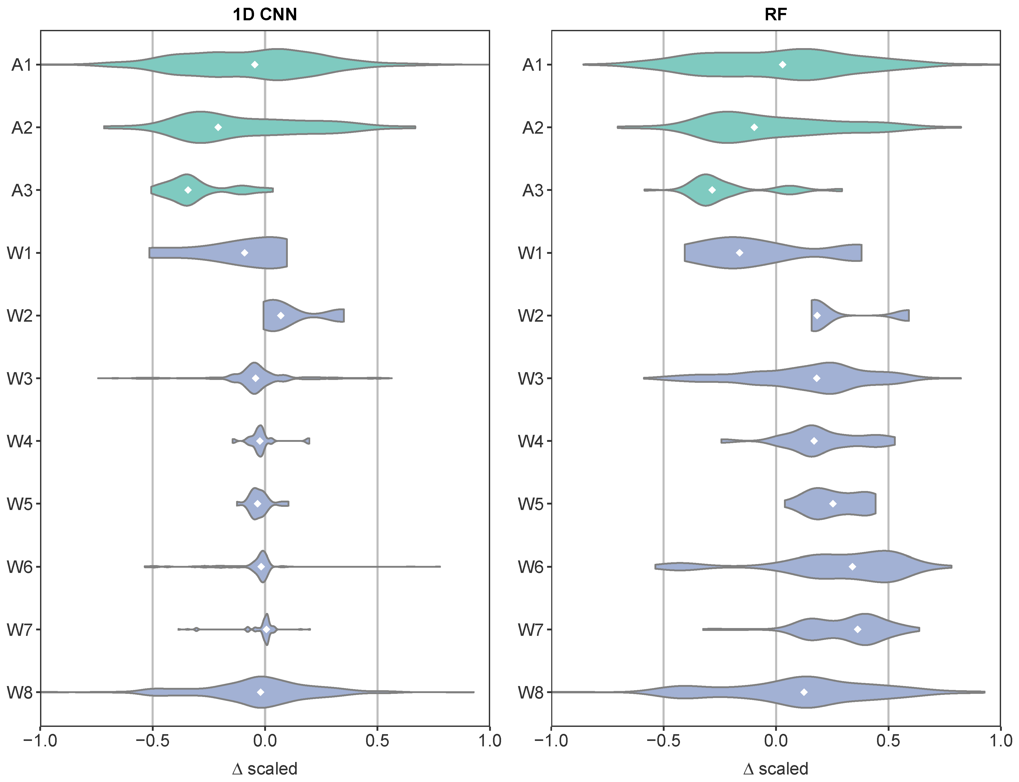
As shown in Figure 9 and Table 5, all ML models can predict the chlorophyll a values of nearly all natural water bodies W1 to W8 satisfyingly. Besides, Figure 10 exemplifies the scaled deviation between the estimation results of the 1D CNN and the RF model and the measured chlorophyll a values of the SpecWa dataset as violin plots. The deviation emphaizes the comparison of the estimation performance concerning all water bodies since we apply a min-max-scaling for each water body individually. This scaling is performed for the measured and estimated chlorophyll a values individually. Eventually, the resulting values are normalized in the range of 0–1 and are independent of the target variable’s unit. Figure 10 provides information about the median of the deviations between the scaled estimated and scaled measured chlorophyll a values (white dot) and the entire distribution of these deviations. The natural water body W2 is an exception concerning the satisfied estimation since only the RF on the SR-Sentinel performs well on this waterbody’s datapoints. However, W8 is an example that is estimated well by both neural networks but only on the SR-EnMAP (see Figure 9 and Figure 10). In addition to W2, the datapoints of A1 are also estimated appropriate by one model, the 1D CNN. This finding refers especially to the SR-EnMAP data (see, for example, Figure 10). A2 and A3 represent the third part of inland water bodies since no ML model can estimate the measured chlorophyll a values satisfyingly. This finding is revealed for the 1D CNN and the RF model when focusing on Figure 10. To sum up, both neural networks and the RF perform well, but their performance depends highly on the individual water bodies and their chlorophyll a concentrations.
4. Discussion
In this section, we discuss the results of Section 3 that we obtained with the applied ML models on the real-world chlorophyll a concentrations of the SpecWa dataset. In Section 4.1, we discuss the estimation performance and applicability of the applied ML models in detail and the models’ estimation performance concerning the two downsampled spectral data. Eventually, we present a comprehensive discussion of the estimation performance for the individual water bodies included in the SpecWa dataset (see Section 4.2).
4.1. Estimation Performance Concerning the Two Downsampled Spectral Data and the Different ML Models
As for the downsampled spectral data shown in Figure 4, the models’ estimation performance on the total SpecWa dataset varies between the well-performing neural networks and the two baseline models on the SR-EnMAP data (see Table 4, Figure 8 and Figure A1). Most models perform similarly and worse on the SR-Sentinel data, as shown in Table 4. Except, the BR performance increases on the SR-Sentinel data since the selected bands are optimized for a multispectral resolution. These worse models’ performances on the SR-Sentinel data can be explained by an information loss due to the coarser spectral downsampling. In addition, the models vary highly in their ability to handle multiple, multicollinear input data and select important features from these data. The information loss is caused by the downsampling of the 1 nm resolution original data to the SR-Sentinel, as shown in Figure 1. In contrast, the SR-EnMAP with 6.5 nm-bandwidth characterizes approximately the spectrum’s original distribution, whereas the SR-Sentinel data no longer presents this characteristic. The SR-EnMAP data includes, for example, the typical chlorophyll a absorption at 685 nm [65] and the following scattering peak 705 nm, which are covered by several bands (see Figure 4). This information is provided by only two broad bands for the SR-Sentinel data. Besides, the chlorophyll a’s origin depending on either green algae or diatoms is only recognizable in the finer resolved SR-EnMAP data. Information about, for example, the water composition of different parameters is missing in the SR-Sentinel. The loss of information impedes the estimation for any data-driven ML model.
Regarding the different models’ performances on the finer resolved SR-EnMAP data, the two baseline models cannot exploit the detailed spectral features (see Table 4, and Figure 8 and Figure A1, right). The RF model, for example, cannot use the high-dimensional WASI-generated simulation data to transfer the linkages of the training process on the unknown SpecWa test dataset as visualized, for example, in Figure 8. This finding is sustained since the RF’s performance on the SR-EnMAP data is even slightly worse than on the more downsampled SR-Sentinel data. In contrast, both neural networks, especially the 1D CNN, benefit strongly from the finer resolution of the SR-EnMAP data, resulting in more spectral input features. This finding is clearly revealed in Figure 8 (left). Therefore, the 1D CNN can learn the linkage between the WASI-generated simulation data and the chlorophyll a values. This DL approach can generalize its learnings on the WASI-generated simulation test dataset, particularly on the entirely unknown SpecWa dataset.
When comparing the two best performing models, the ANN and the 1D CNN, the estimation results reveal that the 1D CNN estimates the chlorophyll a concentrations on the SpecWa dataset better than the ANN in terms of 15.3 p.p for the -score. This outperforming can be explained by the characteristic ability of the 1D CNN to exploit the information implicitly contained in the large number of spectral features of SR-EnMAP better than a conventional ANN. As the 1D CNN architecture includes different filters and kernels, the spectral features’ information is perfectly processed, which seems similar to applying different spectral derivatives [42].
Besides, when focusing on the noise in the real-world dataset, such as the SpecWa dataset, the sun’s spectral signal and the sky glint can be higher than the water-leaving radiance [55]. This noisy part of the signal is reflected on the water surface and is included in the SpecWa test dataset, which affects the estimation performances in Table 4. We have varied the parameters influencing the surface reflection to cover a broad range of occurring real-world conditions during the WASI simulation process. Generally, the ML models need to handle these different illumination conditions as noise. Returning to the comparison of both neural network approaches, the estimation results reveal that the 1D CNN can minimize occurring noise, such as the effect of the absolute reflectance values in the input data. Therefore, the generalization abilities of the 1D CNN ensure the transfer to further spectral data provided by different sensors, illumination conditions, and eventually, distinct water bodies that are prevailed by the underlying estimation task in our study (see, for example, Figure 8, right). The weaker performance of the ANN (see Figure A1, right) can be explained by strongly responding to the noise in the input data.
Finally, we analyze our estimation results and the estimation results provided by a previously conducted study on one part of the SpecWa dataset by Maier and Keller [37]. They have investigated the performance of several shallow ML models to estimate the chlorophyll a concentration with different spectral resolutions. Note that a detailed comparison of the estimation performances is infeasible since the training dataset are entirely different. In the previous study, all ML models have been trained on datapoints of the SpecWa dataset [37]. The SpecWa dataset has been known to the models, which is not the case for our study. Therefore, the overall models’ estimation performance in the previous study is better when regarding the absolute figures. A finding of Maier and Keller [37] is that the models’ performances are only slightly better on the finer resolved SR-EnMAP data. For example, the ANN model performs slightly worse on the SR-Sentinel data than on the SR-EnMAP data (see [37], Table 2). In our study, the ML models show larger differences in their estimation performance between the SR-Sentinel and SR-EnMAP (see Table 4). As for the arising questions addressing the generalization abilities of the models in Maier and Keller [37], they have not been applied to unknown water bodies. Therefore, we assume that these models would perform significantly worse than the models in the underlying study due to the lack of noise and variability generated in our case by the WASI tool.
4.2. Estimation Performance Concerning the Individual Water Bodies
Since the SpecWa dataset consists of chlorophyll a concentrations of eleven different inland water bodies (see, for example, Figure 1), we discuss the applied ML models’ estimation performance concerning these water bodies. In contrast to the commonly applied BR approaches (see, for example, [5,31]), and the more advanced BR approaches for specific water types [19,32], the proposed data-driven ML approaches are not trained on datapoints of the individual water bodies. Our objective is to provide a more generalized approach trained and parametrized on a dataset not necessarily including chlorophyll a values of the target water bodies. This approach differs also from the study of Pahlevan et al. [21], relying on a mixture density model with in-situ data of several inland water bodies. A large amount of training data is required concerning the applicability of a DL approach, which motivates employing simulation data such as the used WASI-generated simulation data. One advantage of data simulation is, for example, the possibility to generate a broader range of chlorophyll a values than appearing in natural water bodies.
Our models’ performance results are given in Section 3, Table 5, Figure 9 and Figure 10. Similar to Section 3, the discussion is structured in three parts. Most of the natural water bodies (W1 to W8) are well estimated by the majority of ML models (see Figure 9) and even on the more downsampled SR-Sentinel data. When focusing on the CNN as the best performing approach (see Table 4) on the En-MAP resolution, we retrieve this assessment based on the deviation distributions of W1-W8 in Figure 10 (left). As shown, the median of the deviations between the scaled estimated and measured chlorophyll a values are allocated around 0. A good estimation of the natural water bodies’ chlorophyll a values implies that the proposed approach to train the ML models on an entirely different and simulated dataset and, subsequently, apply them to an unknown real-world dataset, works well for the entire SpecWa dataset (see Section 4.1) and concerning most of the individual water bodies (see Figure 9). The natural water body W2 is an exception as for the good models’ estimation performance with 6.4 p.p. difference of the best individual RMSE-score. This exception is also illustrated by the severe deviations and filling shapes of the CNN’s and RF’s distributions in Figure 10. In addition to the lowest number of datapoints (8, see Table 1), this exception seems understandable when investigating the water body’s composition. The water level ranges between 0.5 m to 1 m and is low (see Table 1). Therefore, the benthic substrate strongly influences the spectral signature. Besides, small water plants might float on the water surface during the spectral measurements. The latter might cause an overestimation of the chlorophyll a concentration of this specific water body. We have to consider that such effects of polluted water surfaces always appear when measuring real-world water bodies with, for example, dust or pollen cover.
Regarding the artificial water bodies, it can be seen in Figure 9 as well as Table 5 that the ML models’ estimation performances are worse compared to the natural water bodies. This finding can also be retrieved when focusing on the deviation distributions of the artificial water bodies compared to the natural ones in Figure 10. One reason for the worse estimation results can arise since the WASI tool has been originally developed for water bodies with generally lower chlorophyll a concentrations, such as the lake Constance in Germany [29].
Therefore, the WASI-generated simulation training dataset contains only a few higher chlorophyll a values resembling artificial water bodies. Another reason might be that water bodies characterized by broader chlorophyll a concentration ranges are generally more complex to estimate as they contain a variety of substances. These substances overlap in the measured spectral signatures and cannot be deducted easily. Increasing chlorophyll a concentrations evoke a diversity in the inland water body concerning the horizontal distribution and vertical distribution of the water composition. From this perspective, the estimation task is heavily ill-posed for such water bodies, since the in-situ chlorophyll a measurement is taken at a rather specific depth range while the spectral data capture reflectances over the whole water column. Especially for water bodies with higher concentrations, this effect can lead to a higher estimation bias. Against the background of the mentioned aspects, the 1D CNN’s performance on the water body A1 can be slightly revised since most of the datapoints are estimated satisfactory for the chlorophyll a range of 16.3 μg L−1 to 99.6 μg L−1 (see Table 5).
In sum, it is obvious that a stepwise simulation characterizes the WASI-generated data (see Section 2.3) cannot directly correspond to a natural water body. This is the reason why a particular estimation bias is expected (see, for example, Figure 10). Such a bias can be originated due to make assumptions before the simulation process. For example, these assumptions are:
- We simulated the WASI-generated dataset with three different benthic substrates: sand, silt, and a macrophyte species. Natural water bodies have additional materials such as gravel, leaves, or other organic materials that are not covered in the WASI tool.
- In different geogenic regions, a diversity of minerals occur, resulting in distinct reflective properties and colors for, e.g., suspended materials.
- Besides, several phytoplankton species exist, while the WASI-generated simulation data consist only of two species.
Concerning these mentioned aspects and many more, the ML model’s performance, especially the 1D CNN’s, estimate the chlorophyll a of the entire SpecWa dataset successfully and satisfactory for most individual water bodies.
5. Conclusions and Outlook
Continuous monitoring of inland water bodies with RS techniques is highly relevant for many applications and research areas, such as water quality management. To address the topic of monitoring inland water bodies, we focus on estimating the chlorophyll a concentrations of real-world inland water bodies. Therefore, we use chlorophyll a concentrations and spectral data of several water bodies provided by the SpecWa dataset and simulation data generated by the WASI tool. We rely on ML models such as ANN, RF, a BR approach, and a 1D CNN as a DL approach. The innovative aspects of our study can be summarized as follows: (1) a 1D CNN is applied for the first time to estimate chlorophyll a values; (2) since such a DL approach needs a large amount of training data, we train it on WASI-generated simulation data independent from the real-world SpecWa dataset representing the target data. As a pre-processing step, we apply two downsampling approaches resulting in input data’s spectral resolution of SR-Sentinel and the SR-EnMAP. These downsampled data represent the respective satellite missions as a requirement for a possible upscaling approach regarding area-wide monitoring.
First, we train the ML models on the WASI-generated simulation training dataset. This simulation is prepared accordingly and includes a knowledge-based water composition with two origins of the chlorophyll a concentration. Subsequently, all ML models are evaluated on the SpecWa test dataset. The overall best estimation performance on the total SpecWa dataset achieves the 1D CNN with the SR-EnMAP resolution and an , μg L−1, and μg L−1. Downsampling the spectral input data to the SR-Sentinel resolution, decrease the two neural network approaches’ performance. In the case of the 1D CNN, which is also the best estimator, the performance declines by about 19.5 p.p. to . As expected, the ML models benefit the most from the more detailed information in the SR-EnMAP spectral data, including the typical chlorophyll a absorption at 685 nm. When focusing on the individual water bodies of the SpecWa dataset, the most significant differences exist between the natural and artificial water bodies. We discover that the applied models estimate the chlorophyll a concentration of most natural water bodies satisfyingly. However, the estimation performance on the artificial water bodies is worse, mostly explained by the more complex characteristics of these water bodies.
Returning to the initial question, Can ML approaches be trained on a simulated dataset to estimate the chlorophyll a concentration of water bodies not included in the training process?, posed at the beginning, we find the answer composed of the following three parts:
- Yes. ML approaches can be trained on a simulation dataset and can estimate the chlorophyll a concentration of real-world water bodies not included in the training process. The best model is the newly adapted and applied 1D CNN. It can handle noise in the data and different illumination conditions caused by the sun- and sky glint.
- However, the ML models must be provided with appropriate information in the input data. This is the main reason why the estimation performances on the finer resolved SR-EnMAP data are significantly better than on the SR-Sentinal data.
- As for the generalization aspect of the ML models, we demonstrate that it is possible, under specific conditions, that models are trained on a distinct dataset as later applied. Since the DL model performs the best estimation, we take a chance to assume it would perform similarly on another dataset covering the same chlorophyll a values. Indeed, we need to consider the water bodies’ composition.
Considering the last aspect, we point out that the WASI tool is a physical model and always a simplification of the complex reality of a water body. Thus, the estimation performances could be improved by a more complex simulation of the training data, including different influence parameters such as additional algae species or benthic substrates. Another challenge is provided in the SpecWa dataset, since two different devices have been used to measure the reference chlorophyll a values. Combined with the WASI-generated simulation data, the data contains in sum three distinct sensor data.
In total, we conclude that our study is encouraging, mainly as we applied a DL approach that can estimate the chlorophyll a concentration of unknown and independent water bodies. The WASI-generated simulation, in combination with the 1D CNN delivered good results.
Such a choice increases the generalization of ML approaches in the context of inland water monitoring. It provides the first basis for an upscaling approach on real hyperspectral satellite data. Future studies can undertake the presented results and a 1D CNN’s applicability to grip the surface reflectance issues in water quality monitoring. Another possible approach could be to combine different models and prior knowledge to address the chlorophyll a estimation of, for example, deep and shallow waters (depth) or different trophic state (chlorophyll a concentration ranges).
Author Contributions
All authors prepared the methodological concept of this study, the original draft, as well as the editing of the manuscript. P.M.M. designed the software, curated the data, performed the investigation, formal analysis, and validation. P.M.M. and S.K. contributed to the visualization of the data and results. S.K. and S.H. initialized the related research and provided didactic and methodological inputs. All authors contributed to the review of the manuscript. All authors have read and agreed to the published version of the manuscript.
Funding
We acknowledge support by the KIT-Publication Fund of the Karlsruhe Institute of Technology.
Conflicts of Interest
The authors declare no conflict of interest.
Appendix A

Table A1.
Summary of the default WASI simulation parameters (see [56]).
Table A1.
Summary of the default WASI simulation parameters (see [56]).
| Parameter | Standard Value | Unit | Description |
|---|---|---|---|
| C[0] | 0 | μg L−1 | Concentration of phytoplankton class 0 |
| C[1] | 0 | μg L−1 | Concentration of phytoplankton class 1 |
| C[2] | 0 | μg L−1 | Concentration of phytoplankton class 2 |
| C[4] | 0 | μg L−1 | Concentration of phytoplankton class 4 |
| fluo | 0 | chlorophyll a fluorescence quantum yield | |
| S | 0.014 | nm −1 | Exponent of CDOM absorption |
| n | −1 | - | Angström exponent of particle scattering |
| T_W | 25 | °C | Water temperature |
| f | 0.033 | - | f-factor of R |
| Q | 5 | Sr−1 | Anisotropie factor of upwelling radiation |
| z | 0 | m | Sensor depth |
| view | 0 | ° | Viewing angle |
| bbs_phy | 0.001 | m2 mg−1 | Specific backscattering coefficient of phytoplankton |
| f_nw | 0 | - | Fraction of non-water area |
| fA[0] | 0 | - | fraction of bottom type #0 (constant) |
| fA[3] | 0 | - | fraction of bottom type #3 (seagrass) |
| fA[4] | 0 | - | fraction of bottom type #4 (mussel) |
| f_dd | 1 | - | Fraction of direct downwelling irradiance |
| f_ds | 1 | - | Fraction of diffuse downwelling irradiance |
| H_oz | 0.38 | cm | Scale height of ozone |
| alpha | 1.3170 | - | Angström exponent of aerosols |
| beta | 0.2606 | - | Turbidity coefficient |
| WV | 2.500 | cm | Scale height of precipitable water in the atmosphere |
| rho_L | 0.02006 | - | Fresnel reflecance of downwelling radiance |
| rho_dd | 0.03325 | - | Reflection factor of Edd |
| rho_ds | 0.0889 | - | Reflection factor of Eds |
Table A2.
Hyperparameters of the one-dimensional convolutional neural network (1D CNN) (here: CNN) and the artificial neural networks (ANN) with their respective simulated spectral resolutions. The number of filters in the I-th CONV layer is defined as and the number of units in the I-th FC layer is defined as .
| Hyperparameters | CNN + SR-EnMAP | ANN + SP-EnMAP | CNN + SR-Sentinel | ANN + SR-Sentinel |
|---|---|---|---|---|
| Number of epochs | 50 | 50 | 100 | 100 |
| Batch size | 256 | 256 | 256 | 256 |
| Kernel size 1 | 5 | - | 3 | - |
| Kernel size 2 | 4 | - | 2 | - |
| Kernel size 3 | 3 | - | - | - |
| Kernel size 4 | 2 | - | - | - |
| Pooling size | 2 | - | 2 | - |
| Activations | ReLU | ReLU | ReLU | ReLU |
| c1 | 128 | - | 128 | - |
| c2 | 128 | - | 128 | - |
| c3 | 256 | - | - | - |
| c4 | 256 | - | - | - |
| f1 | 200 | 100 | 100 | 100 |
| f2 | 200 | 100 | 100 | 100 |
| Dropout | 0.2 | 0.2 | 0.2 | 0.2 |
| Loss | Mean squared error | |||
| Optimizer | Adam | |||
Figure A1.
Visualization of the estimation results (y-axes) generated by the ANN and the baseline band ratios (BR) model compared to the measured chlorophyll a values (x-axes) on the SpecWa dataset. The natural water bodies W1 to W8 are colored in green while the artificial water bodies are characterized by three different colors: A1 in yellow, A2 in orange, and A3 in blue.

References
- Matthews, M.W. A current review of empirical procedures of remote sensing in inland and near-coastal transitional waters. Int. J. Remote Sens. 2011, 32, 6855–6899. [Google Scholar] [CrossRef]
- Palmer, S.C.; Kutser, T.; Hunter, P.D. Remote sensing of inland waters: Challenges, progress and future directions. Remote Sens. Environ. 2015, 157, 1–8. [Google Scholar] [CrossRef] [Green Version]
- Schaeffer, B.A.; Schaeffer, K.G.; Keith, D.; Lunetta, R.S.; Conmy, R.; Gould, R.W. Barriers to adopting satellite remote sensing for water quality management. Int. J. Remote Sens. 2013, 34, 7534–7544. [Google Scholar] [CrossRef]
- Gitelson, A.A.; Gurlin, D.; Moses, W.J.; Barrow, T. A bio-optical algorithm for the remote estimation of the chlorophyll- a concentration in case 2 waters. Environ. Res. Lett. 2009, 4, 045003. [Google Scholar] [CrossRef]
- Kallio, K.; Kutser, T.; Hannonen, T.; Koponen, S.; Pulliainen, J.; Vepsäläinen, J.; Pyhälahti, T. Retrieval of water quality from airborne imaging spectrometry of various lake types in different seasons. Sci. Total Environ. 2001, 268, 59–77. [Google Scholar] [CrossRef]
- Giardino, C.; Candiani, G.; Zilioli, E. Detecting chlorophyll-a in Lake Garda using TOA MERIS radiances. Photogramm. Eng. Remote Sens. 2005, 71, 1045–1051. [Google Scholar] [CrossRef]
- Koponen, S.; Attila, J.; Pulliainen, J.; Kallio, K.; Pyhälahti, T.; Lindfors, A.; Rasmus, K.; Hallikainen, M. A case study of airborne and satellite remote sensing of a spring bloom event in the Gulf of Finland. Cont. Shelf Res. 2007, 27, 228–244. [Google Scholar] [CrossRef]
- Gons, H.J.; Rijkeboer, M.; Ruddick, K.G. A chlorophyll-retrieval algorithm for satellite imagery (Medium Resolution Imaging Spectrometer) of inland and coastal waters. J. Plankton Res. 2002, 24, 947–951. [Google Scholar] [CrossRef] [Green Version]
- Kutser, T.; Pierson, D.C.; Kallio, K.Y.; Reinart, A.; Sobek, S. Mapping lake CDOM by satellite remote sensing. Remote Sens. Environ. 2005, 94, 535–540. [Google Scholar] [CrossRef]
- Petus, C.; Chust, G.; Gohin, F.; Doxaran, D.; Froidefond, J.M.; Sagarminaga, Y. Estimating turbidity and total suspended matter in the Adour River plume (South Bay of Biscay) using MODIS 250-m imagery. Cont. Shelf Res. 2010, 30, 379–392. [Google Scholar] [CrossRef] [Green Version]
- Maier, P.M.; Keller, S. Machine learning regression on hyperspectral data to estimate multiple water parameters. In Proceedings of the 2018 9th Workshop on Hyperspectral Image and Signal Processing: Evolution in Remote Sensing (WHISPERS), Amsterdam, The Netherlands, 23–26 September 2018; pp. 1–5. [Google Scholar] [CrossRef] [Green Version]
- Dekker, A.; Vos, R.; Peters, S. Comparison of remote sensing data, model results and in situ data for total suspended matter (TSM) in the southern Frisian lakes. Sci. Total Environ. 2001, 268, 197–214. [Google Scholar] [CrossRef]
- Doxaran, D.; Froidefond, J.M.; Castaing, P.; Babin, M. Dynamics of the turbidity maximum zone in a macrotidal estuary (the Gironde, France): Observations from field and MODIS satellite data. Estuarine Coast. Shelf Sci. 2009, 81, 321–332. [Google Scholar] [CrossRef]
- Olmanson, L.G.; Bauer, M.E.; Brezonik, P.L. A 20-year Landsat water clarity census of Minnesota’s 10,000 lakes. Remote Sens. Environ. 2008, 112, 4086–4097. [Google Scholar] [CrossRef]
- Ruiz-Verdú, A.; Simis, S.G.; de Hoyos, C.; Gons, H.J.; Peña-Martínez, R. An evaluation of algorithms for the remote sensing of cyanobacterial biomass. Remote Sens. Environ. 2008, 112, 3996–4008. [Google Scholar] [CrossRef]
- Maier, P.M.; Hinz, S.; Keller, S. Estimation of Chlorophyll a, Diatoms and Green Algae Based on Hyperspectral Data with Machine Learning Approaches. In Proceedings of the 38. Wissenschaftlich-Technische Jahrestagung der DGPF und PFGK18 Tagung in München—Publikationen der DGPF, Band 27, 2018, Munchen, Germany, 7–9 May 2018. [Google Scholar]
- Gholizadeh, M.H.; Melesse, A.M.; Reddi, L. A comprehensive review on water quality parameters estimation using remote sensing techniques. Sensors 2016, 16, 1298. [Google Scholar] [CrossRef] [PubMed] [Green Version]
- Toming, K.; Kutser, T.; Laas, A.; Sepp, M.; Paavel, B.; Nõges, T. First experiences in mapping lake water quality parameters with Sentinel-2 MSI imagery. Remote Sens. 2016, 8, 640. [Google Scholar] [CrossRef] [Green Version]
- Ansper, A.; Alikas, K. Retrieval of chlorophyll a from Sentinel-2 MSI data for the European Union water framework directive reporting purposes. Remote Sens. 2019, 11, 64. [Google Scholar] [CrossRef] [Green Version]
- Cazzaniga, I.; Bresciani, M.; Colombo, R.; Della Bella, V.; Padula, R.; Giardino, C. A comparison of Sentinel-3-OLCI and Sentinel-2-MSI-derived Chlorophyll-a maps for two large Italian lakes. Remote Sens. Lett. 2019, 10, 978–987. [Google Scholar] [CrossRef]
- Pahlevan, N.; Smith, B.; Schalles, J.; Binding, C.; Cao, Z.; Ma, R.; Alikas, K.; Kangro, K.; Gurlin, D.; Hà, N.; et al. Seamless retrievals of chlorophyll-a from Sentinel-2 (MSI) and Sentinel-3 (OLCI) in inland and coastal waters: A machine-learning approach. Remote Sens. Environ. 2020, 240, 111604. [Google Scholar] [CrossRef]
- Carlson, R.E. A trophic state index for lakes. Limnol. Oceanogr. 1977, 22, 361–369. [Google Scholar] [CrossRef] [Green Version]
- Hall, R.I.; Leavitt, P.R.; Quinlan, R.; Dixit, A.S.; Smol, J.P. Effects of agriculture, urbanization, and climate on water quality in the northern Great Plains. Limnol. Oceanogr. 1999, 44, 739–756. [Google Scholar] [CrossRef] [Green Version]
- Kovács, J.; Tanos, P.; Várbíró, G.; Anda, A.; Molnár, S.; Hatvani, I.G. The role of annual periodic behavior of water quality parameters in primary production–Chlorophyll-a estimation. Ecol. Indic. 2017, 78, 311–321. [Google Scholar] [CrossRef] [Green Version]
- Gordon, H.R.; Brown, O.B.; Jacobs, M.M. Computed Relationships Between the Inherent and Apparent Optical Properties of a Flat Homogeneous Ocean. Appl. Opt. 1975. [Google Scholar] [CrossRef] [PubMed]
- Dekker, A.G.; Hoogenboom, H.J.; Goddijn, L.M.; Malthus, T. The relation between inherent optical properties and reflectance spectra in turbid inland waters. Remote Sens. Rev. 1997, 15, 59–74. [Google Scholar] [CrossRef]
- Odermatt, D.; Heege, T.; Nieke, J.; Kneubühler, M.; Itten, K. Water Quality Monitoring for Lake Constance with a Physically Based Algorithm for MERIS Data. Sensors 2008, 8, 4582–4599. [Google Scholar] [CrossRef] [PubMed] [Green Version]
- Schiller, H.; Doerffer, R. Neural network for emulation of an inverse model operational derivation of Case II water properties from MERIS data. Int. J. Remote Sens. 1999, 20, 1735–1746. [Google Scholar] [CrossRef]
- Gege, P. The water color simulator WASI: An integrating software tool for analysis and simulation of optical in situ spectra. Comput. Geosci. 2004, 30, 523–532. [Google Scholar] [CrossRef]
- Gege, P.; Dekker, A.G. Spectral and radiometric measurement requirements for inland, coastal and reef waters. Remote Sens. 2020, 12, 2247. [Google Scholar] [CrossRef]
- Moses, W.J.; Gitelson, A.A.; Berdnikov, S.; Povazhnyy, V. Satellite Estimation of Chlorophyll-a Concentration Using the Red and NIR Bands of MERIS—The Azov Sea Case Study. IEEE Geosci. Remote Sens. Lett. 2009, 6, 845–849. [Google Scholar] [CrossRef]
- Neil, C.; Spyrakos, E.; Hunter, P.D.; Tyler, A.N. A global approach for chlorophyll-a retrieval across optically complex inland waters based on optical water types. Remote Sens. Environ. 2019, 229, 159–178. [Google Scholar] [CrossRef]
- Spyrakos, E.; O’Donnell, R.; Hunter, P.D.; Miller, C.; Scott, M.; Simis, S.G.; Neil, C.; Barbosa, C.C.; Binding, C.E.; Bradt, S.; et al. Optical types of inland and coastal waters. Limnol. Oceanogr. 2018, 63, 846–870. [Google Scholar] [CrossRef] [Green Version]
- Mitchell, T.M. Machine Learning; Machine Learning Department Carnegie Mellon University: Pittsburgh, PA, USA, 1997. [Google Scholar]
- Zhang, Y.; Pulliainen, J.; Koponen, S.; Hallikainen, M. Application of an empirical neural network to surface water quality estimation in the Gulf of Finland using combined optical data and microwave data. Remote Sens. Environ. 2002, 81, 327–336. [Google Scholar] [CrossRef]
- González Vilas, L.; Spyrakos, E.; Torres Palenzuela, J.M. Neural network estimation of chlorophyll a from MERIS full resolution data for the coastal waters of Galician rias (NW Spain). Remote Sens. Environ. 2011, 115, 524–535. [Google Scholar] [CrossRef]
- Maier, P.M.; Keller, S. Application of different simulated spectral data and machine learning to estimate the chlorophyll a concentration of several inland waters. In Proceedings of the 2019 10th Workshop on Hyperspectral Imaging and Signal Processing: Evolution in Remote Sensing (WHISPERS), Amsterdam, The Netherlands, 24–26 September 2019; pp. 1–5. [Google Scholar] [CrossRef] [Green Version]
- Chebud, Y.; Naja, G.M.; Rivero, R.G.; Melesse, A.M. Water quality monitoring using remote sensing and an artificial neural network. Water Air Soil Pollut. 2012, 223, 4875–4887. [Google Scholar] [CrossRef]
- Hafeez, S.; Wong, M.S.; Ho, H.C.; Nazeer, M.; Nichol, J.; Abbas, S.; Tang, D.; Lee, K.H.; Pun, L. Comparison of machine learning algorithms for retrieval of water quality indicators in case-II waters: A case study of Hong Kong. Remote Sens. 2019, 11, 617. [Google Scholar] [CrossRef] [Green Version]
- Syariz, M.A.; Lin, C.H.; Nguyen, M.V.; Jaelani, L.M.; Blanco, A.C. WaterNet: A convolutional neural network for chlorophyll-a concentration retrieval. Remote Sens. 2020, 12, 1966. [Google Scholar] [CrossRef]
- Pu, F.; Ding, C.; Chao, Z.; Yu, Y.; Xu, X. Water-quality classification of inland lakes using landsat8 images by convolutional neural networks. Remote Sens. 2019, 11, 1674. [Google Scholar] [CrossRef] [Green Version]
- Maier, P.; Keller, S. Estimating chlorophyll a concentrations of several inalnd waters with hyperspectral data and machine learning models. ISPRS Ann. Photogramm. Remote Sens. Spat. Inf. Sci. 2019, 4. [Google Scholar] [CrossRef] [Green Version]
- Maier, P.M.; Keller, S. SpecWa: Spectral Remote Sensing Data and Chlorophyll a Values of Inland Waters; GFZ Data Services: Potsdam, Germany, 2020. [Google Scholar] [CrossRef]
- Mobley, C.D.; Sundman, L.K. HYDROLIGHT 5 ECOLIGHT 5; Sequoia Scientific Inc: Bellevue, WA, USA, 2008. [Google Scholar]
- Riese, F.M.; Keller, S. Soil Texture Classification with 1D Convolutional Neural Networks based on Hyperspectral Data. ISPRS Ann. Photogramm. Remote Sens. Spatial Inf. Sci. 2019, IV-2/W5, 615–621. [Google Scholar] [CrossRef] [Green Version]
- Breiman, L. Random Forests. Mach. Learn. 2001, 1, 5–32. [Google Scholar] [CrossRef] [Green Version]
- Keller, S.; Maier, P.M.; Riese, F.M.; Norra, S.; Holbach, A.; Börsig, N.; Wilhelms, A.; Moldaenke, C.; Zaake, A.; Hinz, S. Hyperspectral data and machine learning for estimating CDOM, chlorophyll a, diatoms, green algae and turbidity. Int. J. Environ. Res. Public Health 2018, 15, 1881. [Google Scholar] [CrossRef] [Green Version]
- Guanter, L.; Kaufmann, H.; Segl, K.; Foerster, S.; Rogass, C.; Chabrillat, S.; Kuester, T.; Hollstein, A.; Rossner, G.; Chlebek, C.; et al. The EnMAP spaceborne imaging spectroscopy mission for earth observation. Remote Sens. 2015, 7, 8830–8857. [Google Scholar] [CrossRef] [Green Version]
- Drusch, M.; Del Bello, U.; Carlier, S.; Colin, O.; Fernandez, V.; Gascon, F.; Hoersch, B.; Isola, C.; Laberinti, P.; Martimort, P.; et al. Sentinel-2: ESA’s optical high-resolution mission for GMES operational services. Remote Sens. Environ. 2012, 120, 25–36. [Google Scholar] [CrossRef]
- Keller, S.; Riese, F.M.; Stötzer, J.; Maier, P.M.; Hinz, S. Developing a machine learning framework for estimating soil moisture with VNIR hyperspectral data. ISPRS Ann. Photogramm. Remote Sens. Spatial Inf. Sci. 2018, IV-1, 101–108. [Google Scholar] [CrossRef] [Green Version]
- Riese, F.M.; Keller, S.; Hinz, S. Supervised and Semi-Supervised Self-Organizing Maps for Regression and Classification Focusing on Hyperspectral Data. Remote Sens. 2020, 12, 7. [Google Scholar] [CrossRef] [Green Version]
- Moreno-Torres, J.G.; Raeder, T.; Alaiz-Rodríguez, R.; Chawla, N.V.; Herrera, F. A unifying view on dataset shift in classification. Pattern Recognit. 2012, 45, 521–530. [Google Scholar] [CrossRef]
- Quionero-Candela, J.; Sugiyama, M.; Schwaighofer, A.; Lawrence, N. Dataset Shift in Machine Learning; The MIT Press: Cambridge, MA, USA, 2009. [Google Scholar] [CrossRef] [Green Version]
- Gege, P.; Albert, A. A tool for inverse modeling of spectral measurements in deep and shallow waters. In Remote Sensing of Aquatic Coastal Ecosystem Processes; Springer: Dordrecht, The Netherlands, 2006; pp. 81–109. [Google Scholar] [CrossRef]
- Gege, P.; Grötsch, P. A spectral model for correcting sunglint and skyglint. In Proceedings of the Ocean Optics XXIII, Victoria, Kanada, 23–28 October 2016; pp. 1–10. [Google Scholar]
- Gege, P. WASI5_Manual; Gege: Taipei, Taiwan, 2019. [Google Scholar]
- Beck, R.; Zhan, S.; Liu, H.; Tong, S.; Yang, B.; Xu, M.; Ye, Z.; Huang, Y.; Shu, S.; Wu, Q.; et al. Comparison of satellite reflectance algorithms for estimating chlorophyll-a in a temperate reservoir using coincident hyperspectral aircraft imagery and dense coincident surface observations. Remote Sens. Environ. 2016, 178, 15–30. [Google Scholar] [CrossRef] [Green Version]
- Lehnert, L.W.; Meyer, H.; Obermeier, W.A.; Silva, B.; Regeling, B.; Bendix, J. Hyperspectral data analysis in R: The hsdar package. J. Stat. Softw. 2018, 89. [Google Scholar] [CrossRef] [Green Version]
- Liu, L.; Ji, M.; Buchroithner, M. Transfer learning for soil spectroscopy based on convolutional neural networks and its application in soil clay content mapping using hyperspectral imagery. Sensors 2018, 18, 3169. [Google Scholar] [CrossRef] [PubMed] [Green Version]
- Stevens, A.; Ramirez-Lopez, L.; Stevens, M.A.; Rcpp, L. Package ‘Prospectr’. R Package Version, (2). 2020. Available online: https://www.google.com.hk/url?sa=t&rct=j&q=&esrc=s&source=web&cd=&ved=2ahUKEwi3-_26u-vuAhUIJhoKHWvLDmYQFjAA\egQIAxAC&url=https%3A%2F%2Fcran.r-project.org%2Fweb%2Fpackages%2Fprospectr%2Fprospectr.pdf&usg=AOvVaw3zgdDSp-x6QxrPPFHVyFSV (accessed on 15 February 2021).
- Hu, W.; Huang, Y.; Wei, L.; Zhang, F.; Li, H. Deep convolutional neural networks for hyperspectral image classification. J. Sens. 2015, 2015, 258619. [Google Scholar] [CrossRef] [Green Version]
- LeCun, Y.; Bottou, L.; Bengio, Y.; Haffner, P. Gradient-based learning applied to document recognition. Proc. IEEE 1998, 86, 2278–2324. [Google Scholar] [CrossRef] [Green Version]
- Goodfellow, I.; Bengio, Y.; Courville, A.; Bengio, Y. Deep Learning; MIT Press Cambridge: Cambridge, MA, USA, 2016; Volume 1. [Google Scholar]
- Kingma, D.P.; Ba, J. Adam: A method for stochastic optimization. arXiv 2014, arXiv:1412.6980. [Google Scholar]
- Morel, A.; Prieur, L. Analysis of variations in ocean color. Limnol. Oceanogr. 1977, 22, 709–722. [Google Scholar] [CrossRef]
Figure 1.
Boxplots of the chlorophyll a concentration range for each inland water body individually, and for all water bodies of the SpecWa dataset. The water ID is given in Table 1. The diamonds in the boxes symbolize the respective mean, the lines the respective median value. The lower limit of each box is the 25th percentile (Q1), the upper limit the 75th percentile (Q3) so that the difference builds the interquartile range (IQR). Whiskers extend to and . Any points beyond the whiskers are outliers and are plotted as points.

Figure 2.
Visualization of the spectral data of the two SpecWa water bodies [43]. The solid lines refer to the mean of the waterbodies A1 (blue) and W8 (orange). The brighter area represents the respective standard deviations. In the SpecWa dataset, the radiance reflectance is the normalized ratio between the water leaving radiance combined with the surface reflectance and the incoming irradiance. The corresponding chlorophyll a concentrations and information are given in Figure 1 and Table 1.

Figure 3.
Sampling schema of the selected WASI parameters. Chl a refers to the Chlorophyll a, while are the remaining parameters given in Table 2. I describes the control variable and .
Figure 3.
Sampling schema of the selected WASI parameters. Chl a refers to the Chlorophyll a, while are the remaining parameters given in Table 2. I describes the control variable and .

Figure 4.
Visualization of the two different downsampled spectral resolutions. The spectral resolution of the Sentinel-2 mission (orange) is referred to as SR-Sentinel, and the spectral resolution of the EnMAP mission (blue) as SR-EnMAP. The grey line represents a selected WASI-generated simulation spectrum with a chlorophyll a value of 51 μg L−1, a concentration of suspended materials type I of 7.8 mg L−1, and a sandy bottom substrate. The additonal WASI parameters are set to the (default) values according to Table 2 and Table A1.

Figure 5.
Pre-processing schema for SpecWa dataset (orange) and the WASI-generated simulation dataset (blue). N refers to either 9 spectral input features in the case of the SR-Sentinel resolution or 77 in the case of the SR-EnMAP resolution.
Figure 5.
Pre-processing schema for SpecWa dataset (orange) and the WASI-generated simulation dataset (blue). N refers to either 9 spectral input features in the case of the SR-Sentinel resolution or 77 in the case of the SR-EnMAP resolution.

Figure 6.
Distributions of of the chlorophyll a values between the WASI training subset and the SpecWA dataset. The WASI training set refers to the left y-axis and has about 100 times more datapoints than the SpecWa dataset which is referred to the right y-axis.
Figure 6.
Distributions of of the chlorophyll a values between the WASI training subset and the SpecWA dataset. The WASI training set refers to the left y-axis and has about 100 times more datapoints than the SpecWa dataset which is referred to the right y-axis.

Figure 7.
Flowchart of the 1D CNN for the SR-EnMAP spectral input features during the training process. The network includes convolutional (CONV), fully-connected (FC), and max-pooling (MaxPooling) layers. Besides, a layer with Gaussian noise (Noise) and a dropout layer (dropout) exist. The I-th CONV layer contains filters and the j-th FC layer contains units. At the end of the network, a linear activation function is applied. Adopted from [45]. Adapted with permission from Riese and Keller (2019). Copyright 2019 Riese and Keller.

Figure 8.
Visualization of the estimation results (y-axes) generated by the 1D CNN and the baseline RF model compared to the measured chlorophyll a values (x-axes) on the SpecWa dataset. The natural water bodies W1 to W8 are colored in green while the artificial water bodies are characterized by three different colors: A1 in yellow, A2 in orange, and A3 in blue.

Figure 9.
Visualization of the models’ estimation results based on the RMSE-scores on the different water bodies with the two different downsampled resolutions.
Figure 9.
Visualization of the models’ estimation results based on the RMSE-scores on the different water bodies with the two different downsampled resolutions.

Figure 10.
Visualization of the estimation results on the SR-EnMAP resolved data generated by the 1D CNN (left) and the RF model (right) as the min-max scaled deviation between the estimated and measured chlorophyll a values. The violin plots reveal the median of the deviations between the scaled estimated and scaled measured chlorophyll a values (white dot) and the entire distribution of these deviations.

Table 1.
Summary of the SpecWa dataset [43]. The term ap refers to artificial pond while qp means quarry pont.
Table 1.
Summary of the SpecWa dataset [43]. The term ap refers to artificial pond while qp means quarry pont.
| Water Body | Water ID | Number of Datapoints | Water Depth | Chlorophyll a Range |
|---|---|---|---|---|
| in m | in μg L−1 | |||
| ap castle garden | A1 | 1048 | 1.0 to 2.0 | 16.3 to 99.6 |
| ap KIT | A2 | 116 | 0.5 to 1.0 | 22.2 to 93.0 |
| ap TMB | A3 | 57 | 2.0 to 3.0 | 61.0 to 96.5 |
| old rhine au | W1 | 21 | 2.0 to 3.0 | 4.7 to 9.1 |
| old rhine leopoldshafen | W2 | 8 | 0.5 to 1.0 | 9.8 to 11.0 |
| qp blankenloch | W3 | 494 | 0.5 to 3.0 | 2.4 to 21.0 |
| qp epple | W4 | 42 | 1.0 to 3.0 | 1.6 to 13.0 |
| qp ferma | W5 | 20 | 1.0 to 3.0 | 3.3 to 6.4 |
| qp heide | W6 | 221 | 1.0 to 3.0 | 1.7 to 16.5 |
| qp leopoldshafen | W7 | 105 | 1.5 to 3.0 | 0.0 to 8.7 |
| qp waldstadt | W8 | 485 | 1.5 to 3.0 | 0.0 to 17.0 |
Table 2.
Summary of the relevant Water Color Simulator (WASI) simulation parameters with their respective range. The sampling schema is described in Figure 3. The range and the respective steps define the possible occurring parameter values. For chlorophyll a and the concentration of non-algal particles, a logarithmic scale is chosen.
| WASI Parameter | Range | Standard | Steps | Log Scale | Description |
|---|---|---|---|---|---|
| Chlorophyll a | 1 μg L−1 to 100 μg L−1 | - | 30 | yes | concentration of chlorophyll a |
| C | 0.1 mg L−1 to 100 mg L−1 | 1 | 20 | yes | concentration of non-algal particles type I |
| C | 1 mg L−1 to 20 mg L−1 | 0 | 20 | no | concentration of non-algal particles type II |
| C | 0.1 m−1 to 5 m−1 | 0.1 | 20 | no | CDOM concentration |
| zB | 1 m to 5 m | 2 | 10 | no | water depth |
| Sun | 35° to 65° | 50 | 10 | no | sun position |
| FA1 | 0.1 to 5 | 0 | 10 | no | background type sand |
| FA2 | 0.1 to 5 | 0 | 10 | no | background type silt |
| FA5 | 0.1 to 3 | 0 | 10 | no | background type macrophyte |
| g | 0 Sr−1 to 0.5 Sr−1 | 0.02 | 10 | no | fraction of sky radiance due to direct solar radiation |
| g | 0 Sr−1 to 1 Sr−1 | 0.318 | 10 | no | fraction of sky radiance due to molecule scattering |
| g | 0 Sr−1 to 1 Sr−1 | 0.318 | 10 | no | fraction of sky radiance due to aerosol scattering |
Table 3.
Number of datapoints of the WASI-generated simulation dataset for each of the three subsets.
Table 3.
Number of datapoints of the WASI-generated simulation dataset for each of the three subsets.
| Dataset | % | Number of Datapoints |
|---|---|---|
| Training | 70 | 369,600 |
| Validation | 15 | 79,200 |
| Test | 15 | 79,200 |
Table 4.
Results for the chlorophyll a estimation of all SpecWa inland water bodies.
| Model | SR-EnMAP | SR-Sentinel | ||||
|---|---|---|---|---|---|---|
| R2 in % | RMSE in μg L−1 | MAE in μg L−1 | R2 in % | RMSE in μg L−1 | MAE in μg L−1 | |
| 1D CNN | 81.9 | 12.4 | 6.7 | 62.4 | 19.3 | 14.6 |
| ANN | 66.6 | 16.6 | 9.3 | 54.8 | 23.4 | 17.1 |
| RF | 51.1 | 22.7 | 17.0 | 51.1 | 20.2 | 14.7 |
| BR | 37.9 | 23.0 | 19.3 | 51.5 | 22.3 | 17.8 |
Table 5.
Results for the chlorophyll a estimation of the SpecWa inland water bodies.
| Water ID | Model | SR-EnMAP | SR-Sentinel | ||
|---|---|---|---|---|---|
| RMSE in μg L−1 | MAE in μg L−1 | RMSE in μg L−1 | MAE in μg L−1 | ||
| A1 | 1D CNN | 15.4 | 9.1 | 24.0 | 20.9 |
| ANN | 20.4 | 13.8 | 21.8 | 14.1 | |
| RF | 31.2 | 27.7 | 24.7 | 21.1 | |
| BR | 27.8 | 22.0 | 27.3 | 19.7 | |
| A2 | 1D CNN | 22.0 | 18.2 | 33.1 | 27.5 |
| ANN | 40.9 | 34.6 | 56.7 | 53.3 | |
| RF | 37.6 | 33.4 | 37.0 | 32.6 | |
| BR | 20.0 | 17.2 | 16.6 | 13.7 | |
| A3 | 1D CNN | 37.9 | 36.8 | 43.9 | 42.5 |
| ANN | 35.9 | 34.5 | 33.2 | 32.0 | |
| RF | 29.7 | 27.8 | 57.8 | 57.0 | |
| BR | 38.1 | 37.6 | 18.6 | 16.3 | |
| W1 | 1D-CNN | 2.6 | 2.4 | 4.5 | 3.2 |
| ANN | 3.1 | 3.0 | 3.9 | 3.6 | |
| RF | 6.5 | 6.2 | 4.6 | 4.0 | |
| BR | 17.0 | 16.8 | 16.9 | 16.8 | |
| W2 | 1D CNN | 14.2 | 14.1 | 14.9 | 14.9 |
| ANN | 8.4 | 8.3 | 14.6 | 14.5 | |
| RF | 17.5 | 17.4 | 3.6 | 3.3 | |
| BR | 13.9 | 13.9 | 17.7 | 17.7 | |
| W3 | 1D CNN | 3.9 | 3.0 | 7.8 | 6.4 |
| ANN | 4.0 | 3.0 | 4.5 | 3.4 | |
| RF | 7.5 | 6.6 | 6.8 | 6.0 | |
| BR | 17.8 | 16.8 | 17.8 | 16.9 | |
| W4 | 1D CNN | 3.0 | 2.0 | 3.0 | 2.0 |
| ANN | 4.4 | 3.8 | 3.3 | 2.5 | |
| RF | 2.8 | 1.7 | 2.8 | 1.8 | |
| BR | 9.6 | 8.3 | 10.5 | 7.6 | |
| W5 | 1D CNN | 2.0 | 1.4 | 5.5 | 4.0 |
| ANN | 2.3 | 2.1 | 2.3 | 2.0 | |
| RF | 5.1 | 4.4 | 6.3 | 6.0 | |
| BR | 13.8 | 12.3 | 13.8 | 12.5 | |
| W6 | 1D CNN | 2.8 | 1.6 | 2.9 | 2.2 |
| ANN | 3.2 | 2.0 | 2.7 | 1.6 | |
| RF | 3.3 | 2.7 | 6.0 | 5.6 | |
| BR | 20.0 | 17.2 | 21.7 | 17.2 | |
| W7 | 1D CNN | 2.8 | 1.8 | 2.5 | 2.1 |
| ANN | 5.7 | 4.8 | 3.3 | 2.9 | |
| RF | 2.4 | 2.0 | 4.1 | 3.7 | |
| BR | 21.7 | 21.2 | 20.1 | 19.5 | |
| W8 | 1D CNN | 3.9 | 2.9 | 14.3 | 13.2 |
| ANN | 2.9 | 2.3 | 5.9 | 4.8 | |
| RF | 12.3 | 11.2 | 9.8 | 9.1 | |
| BR | 16.6 | 16.2 | 17.2 | 16.9 | |
Publisher’s Note: MDPI stays neutral with regard to jurisdictional claims in published maps and institutional affiliations. |
© 2021 by the authors. Licensee MDPI, Basel, Switzerland. This article is an open access article distributed under the terms and conditions of the Creative Commons Attribution (CC BY) license (http://creativecommons.org/licenses/by/4.0/).
Share and Cite
MDPI and ACS Style
Maier, P.M.; Keller, S.; Hinz, S. Deep Learning with WASI Simulation Data for Estimating Chlorophyll a Concentration of Inland Water Bodies. Remote Sens. 2021, 13, 718. https://doi.org/10.3390/rs13040718
AMA Style
Maier PM, Keller S, Hinz S. Deep Learning with WASI Simulation Data for Estimating Chlorophyll a Concentration of Inland Water Bodies. Remote Sensing. 2021; 13(4):718. https://doi.org/10.3390/rs13040718
Chicago/Turabian StyleMaier, Philipp M., Sina Keller, and Stefan Hinz. 2021. "Deep Learning with WASI Simulation Data for Estimating Chlorophyll a Concentration of Inland Water Bodies" Remote Sensing 13, no. 4: 718. https://doi.org/10.3390/rs13040718
Note that from the first issue of 2016, this journal uses article numbers instead of page numbers. See further details here.